Conceptual Framework for Accounting
In the realm of engineering, conservation refers to the principle that certain physical quantities remain constant as they move or change form within a system. While many laws of physics are governed by these principles, not every property is conserved. For those that can be created or lost (like specific chemical species or certain types of energy), we use an accounting equation to track their status.
Below is a list of extensive properties that can be counted:
- Total mass
- Mass of individual species
- Mass of individual element
- Total moles
- Moles of individual species
- Moles of individual element
- Total energy
- Thermal energy
- Mechanical energy
- Electrical energy
- Net electrical charge
- Positive electrical charge
- Negative electrical charge
- Linear momentum
- Angular momentum
Attention!
Note that volume is not on this list. Compressible fluids (especially gases) may invalidate volume-based accounting equations. If volumes are given, use density to convert to mass values and then use a mass accounting equation.
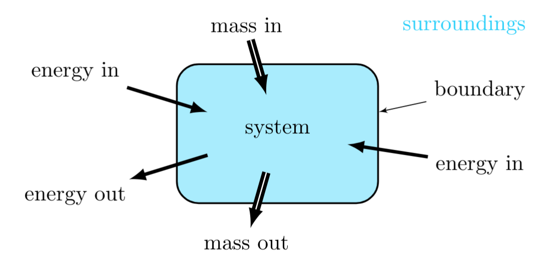
An accounting equation acts as a mathematical ledger. It tracks how an extensive property enters, leaves, is produced, or is used up within a specific boundary over a set timeframe.
All the extensive properties listed above can be counted in accounting equations, but only a subset of these extensive properties is always conserved. Below is a complete list of extensive properties that are conserved in all situations (except nuclear reactions):
- Total mass can be counted for individual species
- Mass of individual element can be counted per element
- Moles of individual element can be counted per element
- Total energy can be counted according to thermal and mechanical energy
- Net charge can be counted across a system
- Linear momentum and Angular momentum can be counted across a system
Process to Use Accounting Equations
To be able to write an accounting statement, three items are necessary:
- The extensive property to be counted must be specified.
- The system and its surroundings must be defined by specifying a boundary.
- A time period must be specified.
Heads up!
Check out Foundations of Transport & Flow.
Forms of Accounting Equations
Mathematically, we illustrate both these concepts:
Accounting:
and Conservation:
or
Accounting equations can be represented in three forms:
- Algebraic
- Differential
- Integral
The following equations will be shown with \( \Psi \) representing any extensive property.
Algebraic Accounting Equations
Algebraic accounting equations are generally applied to extensive properties within a defined system and time period. Algebraic equations can be applied when discrete quantities or “chunks” of extensive property are involved. They cannot be applied when rates or time dependent terms are involved.
Differential Accounting Equations
Differential accounting equations are used when we have flow rates. A flow rate describes the transport of an extensive property over a period of time. We can represent the rate with a dot over the variable, \( \dot{\Psi} \).
Integral Accounting Equations
Integral balances are most useful when trying to evaluate conditions between two discrete time points. Integral accounting equations can be written to incorporate rates of change of an extensive property. When developing an integral balance, you can write the differential balance equation and integrate it between the initial and final times.
Use the table below to ask yourself critical questions about the problem to identify what type of accounting equation is needed.
| Algebraic | Differential | Integral | |
|---|---|---|---|
| Can it incorporate discrete transfer of extensive property? | Yes | No | Sometimes |
| Does it involve a time interval? | Finite | Ongoing | Finite |
| Can it incorporate rates? | No | Yes | Yes |
| What is the dimension of the equation? | Extensive Property | Extensive Property/time | Extensive Property |
Accumulation
The Accumulation term describes the net gain or loss of an extensive property contained within a system. When an Accumulation term is present, the amount of extensive property in the system has changed during the time period of interest. There are two terms that describe the characteristics of the Accumulation term of a system: steady-state or dynamic. Steady-state is a condition in which the values of all the variables in a system (e.g., temperature, pressure, volume, and flow rate) do not change with time, although minor fluctuations about constant mean values may occur. Let us illustrate this by using a photography analogy. If you take multiple, imaginary “snapshots” of a steady-state system over a time period, each snapshot should look the same as the previous one. The initial and final conditions and all the intermediate snapshots of the system are identical or nearly so. The snapshots show that no quantity of the extensive property has accumulated in the system.
A system is in steady-state when its internal conditions (temperature, pressure, etc.) remain constant over time.
- The Misconception: Many believe steady-state means nothing is moving.
- The Reality: A system can have massive amounts of input and output, but as long as the Accumulation is zero, it is in steady-state.
Heads up!
Steady State and Unsteady State build on these concepts in Heat & Mass Transfer.
Example Conservation Problem
Learn More
Need more explanation? See more content in these references.
This content has been adapted from multiple sources including:
- A. Saterbak, K. San, and L. McIntire, (2018). Bioengineering Fundamentals, 2nd Edition.
- Heat, F. O., & Incropera, M. T. F. P. (2001). Fundamentals Of Heat And Mass Transfer.
- Rubenstein, David A, Wei Yin, and Mary D Frame. (2015). Biofluid Mechanics : An Introduction to Fluid Mechanics, Macrocirculation, and Microcirculation, 2nd Edition.