Variables, Units, Dimensions
In biological and medical engineering, the ability to quantify and track physical variables is fundamental to solving complex problems. The majority of figures used in these technical calculations denote the scale of measurable physical properties—variables that are either directly observed or derived by performing arithmetic operations on other data points. Common examples include a system's mass, its spatial length, thermal state, or rate of travel. Generally, these variables are expressed as a combination of a scalar value (the number) and a specific unit (the standard of measurement), such as 6 mL/min.
A unit serves as a standardized, agreed-upon quantity for a specific variable, established through legal standards or scientific convention. It is essential to include these units in all engineering work to ensure the data is meaningful. For instance, stating that "adult human cardiac output is 5" provides no useful information; however, specifying "5 L/min" clearly defines the volume of blood moving through the system over time.
A frequent oversight by novice engineers is the omission of units in their documentation. Some believe they can manage the units mentally without recording them, but this habit often results in calculation errors. For this reason, professional engineers almost never leave units out of their work. Furthermore, complex variables like energy or force are typically broken down into combinations of seven fundamental base quantities. In this context, a "dimension" refers to the qualitative nature of a physical variable rather than a specific numerical scale.
Typical Units in SI and English Systems
Typical Units in SI and English Systems: Dimensions
| Dimension | SI | US |
|---|---|---|
| Length | meter (m) | foot (ft) |
| Mass | kilogram (kg) | pound mass (lb) |
| Time | second (s) | second (s) |
Typical Units in SI and English Systems: State properties
| State property | SI | US |
|---|---|---|
| Pressure | 1 Pa = N/m\( ^2 \) = J/m\( ^3 \) | Pounds per square inch (PSI)|
| Volume | m\( ^3 \) | ft\( ^3 \) |
| Temperature | degrees Celcius (\( ^{\circ} \)C) | degrees Fahrenheit (\( ^{\circ} \)F) |
| Absolute Temperature | Kelvin (K) | degree Rankine (\( ^{\circ} \)R) |
| Internal Energy, Enthalpy | Joules (J) | British thermal Unit (Btu) |
| Newton-meter (N\( \cdot \)m) | Foot-pound force (ft\( \cdot \)lbf) | |
| Entropy | (J/K) | Btu/\( ^{\circ} \)R |
Useful Conversions
Pressure
Temperature
Energy
Extensive and Intensive Properties
Physical characteristics are categorized as either extensive or intensive based on how they react to changes in system size.
Extensive Properties
An extensive property is a value that represents the total sum of all non-interacting parts within a system. Consequently, the magnitude of an extensive property is directly tied to the dimensions of the system or the amount of matter present. To identify one, ask if the value would double or drop by half if the system's size were adjusted accordingly. If the value changes with the scale, it is extensive. These properties are unique because they can be "counted" or tracked in balance equations. Examples include total mass, molar amounts, specific chemical species, electrical charges, momentum, and various forms of energy.
Intensive Properties
Conversely, an intensive property remains constant regardless of the system's total size or the volume of the sample collected. If you were to divide or multiply the system’s scale, an intensive property would stay exactly the same. Because these values do not scale with the amount of material, they cannot be used for counting in conservation or accounting formulas. Common intensive properties include temperature, pressure, density, and the fractional concentration of components (mass or mole fractions) within a mixture. For example, if 1 kg of water is at 25°C and you add another kilogram of water at the same temperature, the resulting 2 kg of water remains at 25°C. Since the temperature does not double, it is classified as intensive.
Scalar and Vector Properties
Physical variables are further divided into scalars and vectors. A scalar is a quantity that is fully described by its magnitude alone. A vector, however, requires both a magnitude and a specific spatial orientation. Vectors must be defined in relation to a fixed starting point or origin within a coordinate system (such as Cartesian, cylindrical, or spherical). In technical literature, vectors are often identified by an arrow symbol above the variable. Mathematically, multiplying two scalars results in another scalar. However, multiplying a scalar by a vector produces a new vector; if the scalar is positive, the direction remains the same, whereas a negative scalar reverses the direction. A classic application of this is multiplying mass (a scalar) by acceleration (a vector) to determine force (a vector).
Extra!
Check out this great resource for unit conversions: Engineering ToolBox
Vectors Bases
To describe vectors mathematically, we write them as a combination of basis vectors. An orthonormal basis is a set of two (in 2D) or three (in 3D) basis vectors which are orthogonal (have 90° angles between them) and normal (have length equal to one). We will not be using non-orthogonal or non-normal bases.
Any other vector can be written as a linear combination of the basis vectors:
The numbers \(a_1, a_2, a_3\) are called the components of \( \vec{a} \) in the \( \,\hat{\imath}, \hat{\jmath}, \hat{k} \) basis. If we are in 2D then we will only have two components for a vector.
Length of Vectors
The length of a vector \( \vec{a} \) is written either \( \| \vec{a} \| \) or just plain \(a\). The length can be computed using Pythagorus’ theorem:
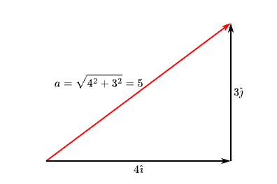
Computing the length of a vector using Pythagorus' theorem.
Some common integer vector lengths are \( \vec{a} = 4\hat\imath + 3\hat\jmath \) (length \(a = 5\)) and \( \vec{b} = 12\hat\imath + 5\hat\jmath \) (length \(b = 13\)).
Learn More
Need more explanation? See more content in these references.
This content has been adapted from multiple sources including:
- A. Saterbak, K. San, and L. McIntire, (2018). Bioengineering Fundamentals, 2nd Edition.
- Heat, F. O., & Incropera, M. T. F. P. (2001). Fundamentals Of Heat And Mass Transfer.
- Rubenstein, David A, Wei Yin, and Mary D Frame. (2015). Biofluid Mechanics : An Introduction to Fluid Mechanics, Macrocirculation, and Microcirculation, 2nd Edition.