General Heat Transfer Governing Equation
The governing heat equation is derived from an energy balance applied to a differential control volume and Fourier's Law. It includes all possible mechanisms that can contribute to heat transfer in a system, and encapsulates the combined effects of energy storage, conduction, convection, and internal heat generation, and allows the prediction of the temperature profile within the system. It combines the energy balance over a system with Fourier's Law.
It can be used to describe the temperature in a material in any kind of heating or cooling situation. The result is a function that is valid at all points in a control volume, at all times (e.g., \( f(x,y,z,t) \)). While heat transfer can occur in three dimensions, it is simplified here to be solved with heat flowing only in one direction (x,r). The governing heat equation can be written in Cartesian or radial coordinates.- \( T \) = temperature \( [K] \)
- \( x \) = position (one-dimensional flow) \( [m] \)
- \( t \) = time \( [s] \)
- \( u \) = fluid velocity \( [\frac{m}{s}] \)
- \( Q \) = heat generated per volume \( [\frac{W}{m^3}] \)
- \( k \) = thermal conductivity \( [\frac{W}{mK}] \)
- \( \rho \) = density \( [\frac{kg}{m^3}] \)
- \( c_p \) = specific heat \( [\frac{J}{kg*K}] \)
In practice, many problems involve simplifying assumptions (e.g., system at steady state, no bulk flow in the system, or no internal heat generation), which allow certain terms to be removed. The meaning of each term and the conditions under which it should be retained or dropped are summarized below.
| Term | What is it? | When do I keep it? | When can I drop it? |
|---|---|---|---|
| \( \frac{\partial T}{\partial t} \) | Stored energy | Unsteady state, \( T \) changing with time (transient) | Steady state (constant \( T \)) |
| \( u\frac{\partial T}{\partial x} \) | Bulk flow (Convection) | Fluid flow | No flow (solid) |
| \( \frac{k}{\rho c_p} \frac{\partial ^2 T}{\partial x^2} \) | Conduction | Almost always | No conduction (no temperature gradient) |
| \( \frac{Q}{\rho c_p} \) | Generation | Conversion of energy in the system | No generation/heat source |
Table 1: Governing equation terms and simplifications.
Boundary and Initial Conditions
To obtain a particular solution, we must solve the general governing equation utilizing known quantities called boundary conditions (BCs, which describe heat transfer at particular surfaces and interfaces) as well as initial conditions (ICs, for unsteady state or time-dependent problems).
Surface Temperature Specified (BC)
Temperature at the surface can be specified as a constant or a function of time.
- For example: \( T(x=L)=100 K \)
- Example of BC in Problem 4.11: The leg is often cooled in a refrigerant prior to surgery to reduce the blood flow even further and numb the nerve endings to make surgery and recovery easier for the patient. Assume the skin temperature is equal to the refrigerant temperature, which is unchanged by the cooling process.
Surface Heat flux Specified (BC)
Heat flux at the surface is specified as a constant or a function of time. There are two special cases for this boundary condition:
- Insulated Condition: the surface is highly insulated so the flux at the surface can be estimated as zero. For example: \( \frac{\partial T}{\partial x}(x=L)=0 \).
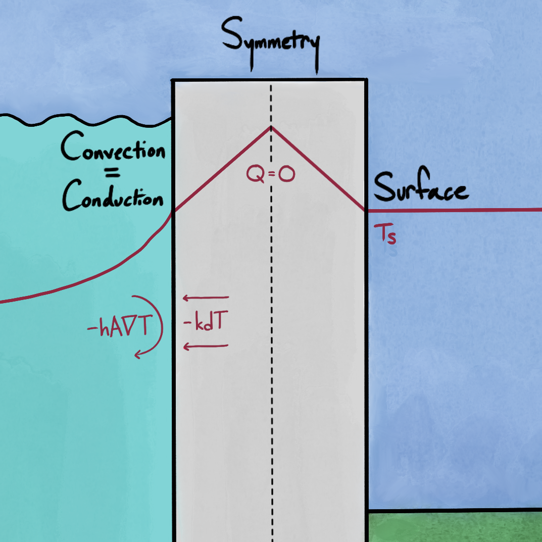
- Symmetric Condition: the system has symmetric geometry making the flux at the centerline equal to zero. For example: \( \frac{\partial T}{\partial x}(x=0)=0 \).
- Example of BC in Problem 4.11: The leg is often cooled in a refrigerant prior to surgery to reduce the blood flow even further and numb the nerve endings to make surgery and recovery easier for the patient. The leg can be modeled as a cylinder with constant thermal properties in the radial direction. The metabolic heat generation is slowed by the cooling, but is still present uniformly throughout the leg.
Convection at the Surface (BC)
When there is a fluid at the surface, the flow of heat due to conduction can be set equal to the flow due to convection. There is one special case for this boundary condition:
- When h is large, the system looks like the boundary condition where the surface temperature can be specified as 0.
Initial Condition
An initial condition provides information about what is happening within the system (e.g., the temperature) at the start of our period of interest. This is necessary to solve a time-varying (i.e., unsteady state) problem.
- For example: \( T(t=0)=T_i \)