Laplace Transform
What Are Laplace Transformations?
This is another frequency mapping technique that can be easier to use than Fourier transforms, as they use a table and map certain identities to known transforms. Laplace transforms are used to describe transfer functions since the Laplace domain makes transfer function math a lot easier. When a signal is affected by a transfer function, the input is simply multiplied by the transfer function to produce the output, which is a much simpler operation to complete than convolution in the time domain.
Quick Facts About Laplace Transforms
Laplace transforms:
- Are linear.
- Use \( s \) as their variable (a complex number).
- Require initial conditions.
- Can be performed forwards and backwards (or inversely) without losing information.
| Time Domain: f(t) | Laplace Domain: F(s) |
|---|---|
| Impulse \( \delta(t) \) | \( 1 \) |
| Step \( 1(t) \) | \( \frac{1}{s} \) |
| Ramp \( t \) | \( \frac{1}{s^{2}} \) |
| \( t^{n} \) | \( \frac{n!}{s^{n+1}} \) |
| \( e^{-at} \) | \( \frac{1}{s+a} \) |
| \( te^{-at} \) | \( \frac{1}{(s+a)^2} \) |
| \( \sin(\omega t) \) | \( \frac{\omega}{s^2+\omega^2} \) |
| \( \cos(\omega t) \) | \( \frac{s}{s^2+\omega^2} \) |
| \( e^{-at}\sin(\omega t) \) | \( \frac{\omega}{(s+a)^2+\omega^2} \) |
| \( e^{-at}\cos(\omega t) \) | \( \frac{s+a}{(s+a)^2+\omega^2} \) |
Where \( t \geq 0 \) for all time domain functions.
Common Signals In Laplace Domain
| Function | Plot | Time Domain: f(t) | Laplace Domain: F(s) |
|---|---|---|---|
| Step | 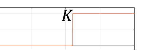 | \( x(t) \begin{cases} &0\ \ \ \ t\leq 0\\ &K\ \ \ t>0\\ \end{cases} \) | \( \frac{K}{s} \) |
| Ramp | 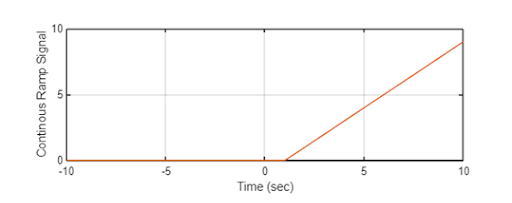 | \( r(t) \begin{cases} &0\ \ \ \ \ \ t\leq 0\\ &Kt\ \ \ t>0\\ \end{cases} \) | \( \frac{K}{s^2} \) |
| Impulse | 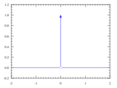 | \( \delta(t) \) | \( 1 \) |
| Pulse/Rectangle | 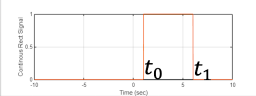 | \( rect(t) = \begin{cases} &1\ \ \ t_0<t<t_1\\ &0\ \ \ else\\ \end{cases} \) | \( \frac{1}{s}-\frac{e^{-t_{1}s}}{s} \) |
Laplace Transform With Other Domains
| Time ==> Laplace | Laplace Transform |
| Laplace ==> Time | Inverse Laplace Transform |
| Laplace ==> Frequency | Steady State \( s = j\omega \) |
| Frequency ==> Laplace | No Initial Conditions \( j\omega = s \) |
Interactive Laplace Transform Lab
Experiment with continuous-time signals \( f(t) \) and their corresponding Laplace domain representations \( F(s) \) in real time. Select canonical waveforms from the transform table (such as exponential decay, damped sinusoids, and rectangular pulses), adjust the decay factor \( a \) (controlling real pole location \( \sigma = -a \)) and oscillation frequency \( \omega \) (controlling imaginary pole location \( \pm j\omega \)), or directly drag the poles ✕ across the complex plane. Observe how pole locations directly govern time-domain envelope decay, oscillations, and the Region of Convergence (ROC).