Stability
In linear systems and controls, eigenvalues are the solutions to the characteristic equation found by setting the denominator of a transfer function to zero (also referred to as the roots or poles of the system). The locations of these eigenvalues directly govern whether a system is stable, unstable, or marginally stable over time.
What Is Stability?
When we have a system, there are three outcomes: stable, unstable, and marginally stable. Stable means that the system reaches a steady state, whereas unstable describes a system that explodes to infinity. Marginally stable is a distinct case where the system does not reach a steady state but remains bounded, such as a sinusoid.
Eigenvalues are scalar values that tell us the long-term behavior and stability of a system. Additionally, Eigenvalues, which are represented with the Greek letter lambda (\( \lambda \)), can be found for a system in the time-domain, \( y(t) \), and in the Laplace domain, \( g(s) \). In the Laplace domain, the eigenvalues are also called poles. The table below corresponds eigenvalues with their system stability.
| Eigenvalues | System Response |
|---|---|
| \( \lambda < 0 \) (real, negative) | Decays towards zero; the system is stable. |
| \( \lambda > 0 \) (real, positive) | Grows exponentially; the system is unstable. |
| \( \lambda = 0 \) | Does not reach steady state but remains bounded; the system is marginally stable. |
| \( \lambda = a \pm bi \) (complex conjugate with imaginary and real values) | System oscillates; the system is either stable or unstable depending on the real component (positive or negative). |
Determining System Stability from Transfer Functions
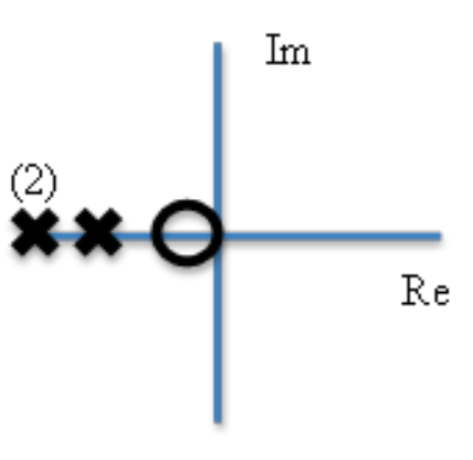
Using the Laplace transfer function, we can solve for the roots of the numerator and denominator polynomials to determine system behavior. For example, consider the transfer function:
For numerator, \( s = -0.5 \) (zero). For denominator, \( s = -3 \) (double pole), \( -2 \) (pole). These values are also referred to as Eigenvalues. Since the poles are all negative, the system is stable.
Determining System Stability from Graphs
| Graph | System Stability |
|---|---|
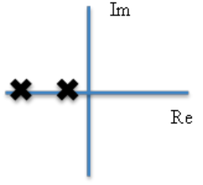 | Stable: If all of the poles are in the left-hand plane, the system is stable. This means that it has negative real numbers and may or may not have an imaginary value as shown in the graph below. If the pole is all real numbers, the system will be a decaying exponential. If the pole is a complex number, the system will be an oscillating decay. Either way, the system is stable. |
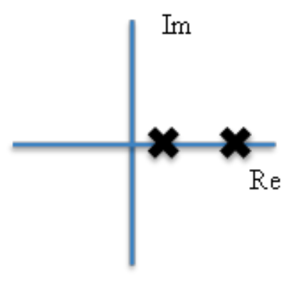 | Unstable: If any of the poles are in the right-hand plane, the system is unstable. This means that at least one pole has a positive real number and may or may not have an imaginary value as shown. |
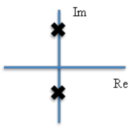 | Marginally Stable: If any of the poles on the imaginary y-axis, the system is marginally stable. This means that at least one pole has a 0 real number and may or may not have an imaginary value. One common example is a sinusoid system. |
Interactive Stability Simulator
Experiment with the interactive MATLAB-style simulator below. Drag the pole ✕ across the complex plane, adjust the sliders, or select presets to observe how the real component \( \sigma \) and imaginary component \( \omega \) directly dictate the stability and time-domain response \( y(t) \).
Interactive System Stability Lab
Drag the pole ✕ on the complex s-plane or use the sliders to watch how pole locations control real-time stability and impulse response.
The pole has a negative real part (σ < 0), causing exponential decay (eσt → 0). Nonzero imaginary components (ω ≠ 0) create oscillations. The system reaches steady state and is Stable.