Conduction
Conductive (or diffusive) heat transfer is the transport of thermal energy through direct contact. Energy is transferred "down" a temperature gradient from high to low based on the Second Law of Thermodynamics. A higher temperature is correlated with higher molecular energy.
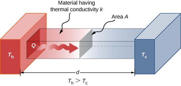
Fourier’s Law is used to describe conductive heat transfer:
where
- \( q^{''}_x \) = flux (rate of heat flow per unit area) \( [\frac{W}{m^2}] \)
- \( q_x \) = rate of heat flow in the x-direction \( [W] \)
- \( A \) = surface area perpendicular to the direction of heat flow \( [m^2] \)
- \( T \) = temperature of the medium at x \( [K] \)
- \( k \) = thermal conductivity of the medium \( [\frac{W}{mK}] \)
Thermal conductivity k describes how well a material can conduct heat.
Heads Up!
Always keep track of your units. To convert between Fahrenheit, Celsius, and Kelvin:
Steady State
In steady state heat conduction, temperature does not change over time. However, temperature can change with position, and this gradient drives the transfer of heat. We can consider three examples of steady state heat conduction.
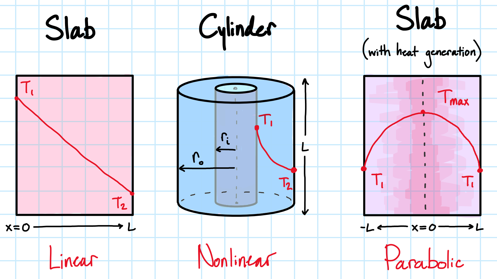
A slab has a linear temperature profile at steady-state. If the slab has a constant internal heat generation, it yields a parabolic temperature profile instead. Cylindrical and spherical geometries have nonlinear temperature profiles, as the cross-sectional area varies with position through the object.
Table 1: Steady-state temperature, flow, and thermal resistance in slab (Cartesian), cylindrical, and spherical geometries.
| Geometry | Temperature Profile | Heat Flow | Thermal Resistance |
|---|---|---|---|
| Slab | \( T=(T_{2}-T_{1})\frac{x}{L}+T_{2} \) | \( q_{x}=\frac{T_{1}-T_{2} }{\frac{L}{kA}} \) | \( \frac{L}{kA} \) |
| Hollow Cylinder | \( T=T_{i}-\frac{T_{i}-T_{0}}{ln(r_{0}/r_{i}}ln(\frac{r}{r_{i}}) \) | \( q_{r}=\frac{T_{i}-T_{0}}{\frac{ln(r_{0}/r_{i})}{2 \pi kL}} \) | \( \frac{ln(r_{0}/r_{i})}{2 \pi kL} \) |
| Hollow Sphere | \( T = T_{i}-(T_{i}-T_{0}) \frac{r-r_{i}}{r_{0}-r_{i}} \frac{r_{0}}{r} \) | \( q_r = \frac{T_{i}-T_{0}}{(r_{0}-r_{i})(4 \pi r_{0} r_{i} k)} \) | \( \frac{r_{0}-r_{i}}{4 \pi r_{0} r_{i} k} \) |
Composite Materials
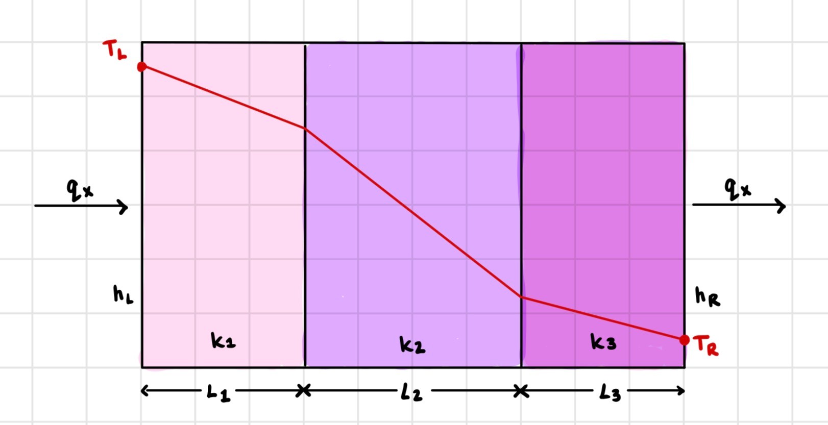
With a composite slab, convection occurs on either side of the slab while conduction occurs within the layers of the slab.
Heat flow can be calculated by temperature differences and thermal resistances:
where
- \( q_{x} \) = heat flow \( [W] \)
- \( T_L \) = temperature on the left side of the slab \( [K] \)
- \( T_R \) = temperature on the right side of the slab \( [K] \)
- \( L \) = length of respective slab layers (1, 2, and 3) \( [m] \)
- \( h \) = convective heat transfer coefficient of the respective sides of the slab \( [\frac{W}{m^2 K}] \)
- \( A \) = cross sectional area of slab \( [m^2] \)
- \( k \) = thermal conductivity of respective slab layers (1, 2, and 3) \( [\frac{W}{mK}] \)
When the resistances are in series:
- Heat flows through each slab layer sequentially.
- The rate of heat flow is the same through each resistance layer.
- Thermal resistance of each layer can be added up into one effective resistance.
When the resistances are in parallel:
- Heat divides and flows through each slab layer simultaneously.
- The total rate of heat flow is the rate of heat flow of each layer added together.
- Thermal resistance of each layer adds like electrical resistances in parallel.
Review
Thermal resistance can be added in series and parallel like electrical resistance:
Series:
Parallel:
or
Unsteady State
In unsteady state (also called nonsteady state or transient) heat conduction, temperature changes over time. There are three situations of unsteady state heat conduction that will be examined here. First, characteristic length and Biot will need to be defined.
Characteristic Length
The Characteristic Length (\( L \)) of an object is its path of least resistance. In other words, it is the shortest distance the heat must travel to escape the object.
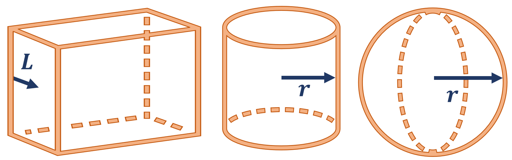
Table 2: Characteristic length for slab, cyclindrical, and spherical geometries.
| Geometry | Characteristic Length (\( L \)) |
|---|---|
| Infinite Slab | \( \frac{1}{2} \) thickness |
| Thin Cylinder | \( \frac{1}{2} \) thickness |
| Tall Cylinder | Radius |
| Sphere | Radius |
Biot Number
The Biot number (\( Bi \)) is used to determine if the internal resistance within an object is negligible. If it is negligible, this means there is very little temperature variation within the solid. It is is calculated as a fraction of internal and external resistance:
where
- \( h \) = convective heat transfer coeffiecent \( [\frac{W}{m^{2} K}] \)
- \( L \) = characteristic length \( [m] \)
- \( k \) = thermal conductivity of the medium \( [\frac{W}{mK}] \)
If \( Bi<0.1 \), the internal resistance can be ignored, and no spatial variation in temperature can be assumed (i.e., temperature changes only as a function of time). If \( Bi>0.1 \), the internal resistance cannot be ignored due to spatial variation in temperature within the solid.
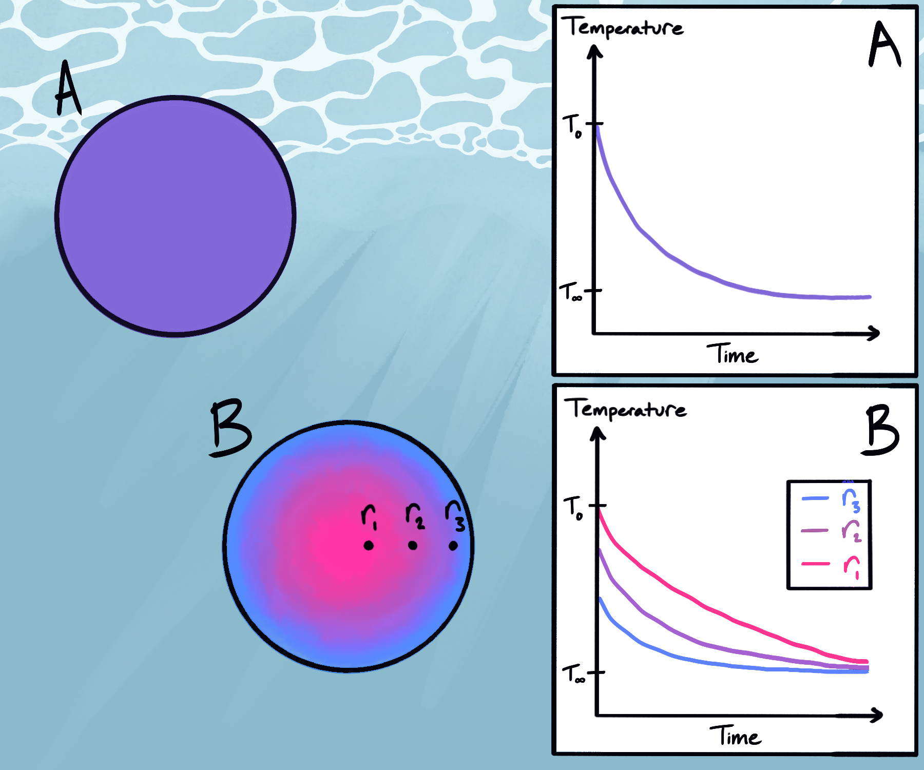
No Spatial Variation in Temperature
If temperature does not vary in all 3 spatial directions and only varies with time, a lumped parameter approximation can be used. When internal resistance is very low compared to the external resistance, the total resistance can be assumed to be external resistance and the temperature will not vary inside the object.
To determine if there is no spatial variation in temperature, use the Biot Number!
- If \( Bi < 0.1 \), the lumped parameter approximation can be used
Lumped Parameter Solution:
where
- \( T \) = surface temperature of the solid \( [K] \)
- \( T_{i} \) = initial temperature of the solid \( [K] \)
- \( T_{\infty} \) = temperature of bulk fluid or air \( [K] \)
- \( t \) = time \( [s] \)
- \( m \) = mass of the solid \( [kg] \)
- \( c_{p} \) = specific heat of the solid \( [\frac{J}{kgK}] \)
- \( h \) = convective heat transfer coeffiecent of fluid or air \( [\frac{W}{m^{2} K}] \)
- \( A \) = area of the solid \( [m^{2}] \)
Spatial Variation in Temperature
If the internal resistance is significant, temperature variation inside cannot be ignored. There are a couple methods to analyze systems with spatial and time variation of temperature. For systems with finite geometry, we can use the series solution.
Use the Biot Number to determine if internal resistance is significant!
- If \( Bi > 0.1 \), internal resistance is significant
Series Solution:
You can solve the series solution two different ways: numerically or using a Heisler Chart.
Heisler Charts are used to describe the relationship between the temperature, position, and time variables. It plots the 1st term of the series solution. The 1st term of the series solution is sufficient after “long times”.
The Fourier Number is used to determine “long times” after initial:
where
- \( \alpha = \frac{k}{\rho c_{p}} \) = thermal diffusivity \( [\frac{m^{2}}{s}] \)
- \( t \) = time \( [s] \)
- \( L \) = Characteristic Length \( [m] \)
In order to use the Heisler Chart your system must satisfy the following:
- Uniform initial temperature, \( T_{i} \)
- Constant boundary fluid temperature, \( T_{\infty} \)
- Perfect slab, cylinder, or sphere geometry
- Far from edges
- No heat generation \( (Q=0) \)
- Constant thermal properties \( (k, \rho, c_{p}) \)
- Long time after initial: \( F_{o} > 0.2 \)
If the system does not satisfy the Heisler Chart conditions, the solution has to be found numerically.
Learn More!
To learn how to use the Heisler Chart, visit the Reference Library & Resources Page!
Near the Surface of a Large Body
The second method to analyze systems with spatial and time variation of temperature \( (Bi > 0.1) \) is for short time and/or thick material. This can be solved with the semi-infinite region solution.
Material is considered thick if it extends to infinity in two directions and has a single identifiable surface. It can be calculated by:
where
- \( L \) = Characteristic Length \( [m] \)
- \( t \) = time \( [s] \)
- \( \alpha \) = thermal diffusivity \( [\frac{m^{2}}{s}] \)
Semi-infinite Region Solution:
where
- \( T \) = temperature at x \( [K] \)
- \( T_{i} \) = tempurature far from the surface\( [K] \)
- \( T_{s} \) = surface temperature \( T [K] \)
- \( x \) = specified location \( [m] \)
- \( \alpha \) = thermal diffusivity \( [\frac{m^{2}}{s}] \)
- \( t \) = time \( [s] \)
For Reference!
A chart with the error function (erf) is provided on the formula sheet found on the Reference Library & Resources Page!
Solutions Summary Table
Table 3: Summary of conditions and equations for lumped parameter, series, and semi-infinite solution.
| Situation | Biot Number | Thickness | Solution Equation |
|---|---|---|---|
| Lumped | \( <0.1 \) | \( L \leq 4\sqrt{\alpha t} \) | \( \frac{T-T_{\infty}}{T_{i} - T_{\infty}} = exp(- \frac{t}{\frac{mc_{p}}{hA}}) \) |
| Series | \( >0.1 \) | \( L \leq 4\sqrt{\alpha t} \) | \( \frac{T - T_{s}}{T_{i} - T_{s}} =\sum_{n=0}^{\infty} \frac{4(-1)^n}{(2n+1)\pi} \cos\left(\frac{(2n+1)\pi x}{2L}\right)\exp\left[-\left(\frac{(2n+1)\pi}{2}\right)^2 \frac{\alpha t}{L^2}\right] \) |
| Semi-Infinite | \( >0.1 \) | \( L \geq 4\sqrt{\alpha t} \) | \( \frac{T-T_{i}}{T_{s} - T_{i}} = 1 - erf[\frac{x}{2\alpha t}] \) |