Transfer Functions

What Are Transfer Functions?

Transfer functions are the Laplace domain representation of signal modification in a system where the input = u(t) or U(s), output = y(t) or Y(s), and the transfer function = h(t) or H(s) where "s" indicates a function in the Laplace domain. The transfer function H(s) is defined as the ratio between the output and the input:

Essentially this means that the output is equal to the input multiplied by the transfer function:

+

Example Problem: Finding System Output from a Block Diagram #tf_simple

Figure 1. A single-block system with an input and transfer function.

Solution +

Using the relationship \( Y(s) = H(s) cdot U(s) \):

$$ Y(s) = \frac{4}{(s+3)(s+4)} $$

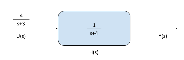
Another important consideration of transfer functions is that they can be combined and simplified, similar to the components of an electrical circuit. Transfer functions in series are multiplied together, while branches that are in parallel are added or subtracted depending on the summing junction signs.

+

Example Problem: Single Block Representation of Combined Systems #tf_combined

Figure 2. Multiple transfer function blocks arranged in series and parallel branches.

Solution +

Combining the series cascade and parallel difference gives the overall transfer function:

$$ H(s) = G_{1}G_{2}(G_{4}G_{5}-G_{3}) $$

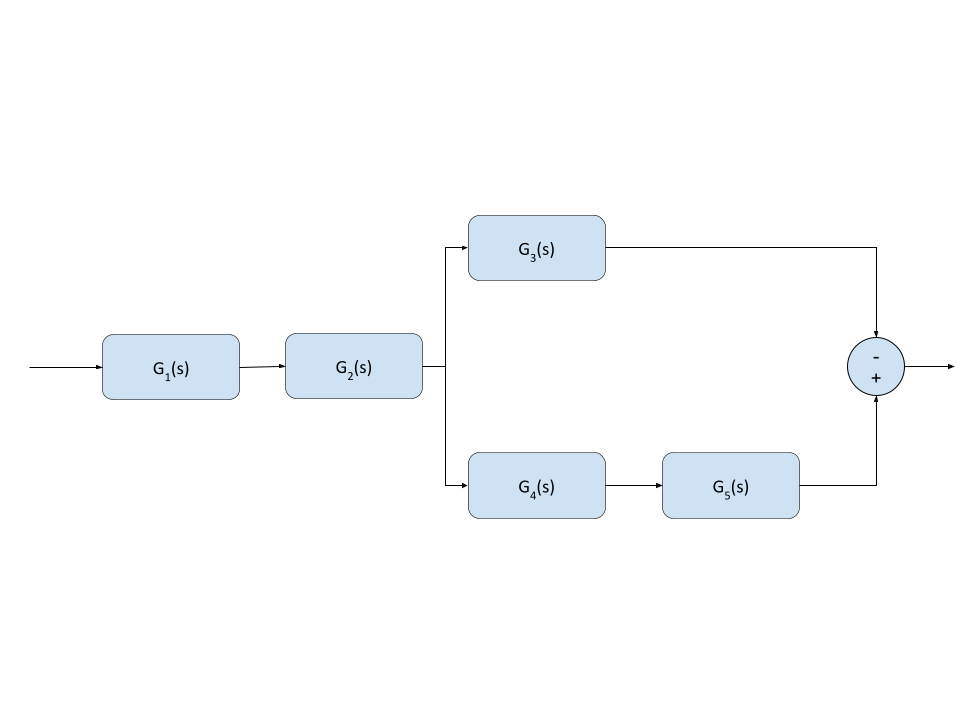
Try practicing with systems that combine these aspects, and use the table of common Laplace transforms (here) to convert your frequency-domain outputs back to the time domain.