Stability

What is Stability?

When we have a system, there are three outcomes: stable, unstable, and marginally stable. Stable means that the system reaches a steady state whereas unstable describes a system that explodes to infinity. Marginally stable is a more unique case where the system does not reach a steady state but remains bounded, such as a sinusoid.

Determining System Stability From Graphs

Using the Laplace Transfer function, we plot this on a graph where the x-axis is real numbers and the y-axis is imaginary numbers. For example, we have the equation:

$$ G(s) = \frac{s+0.5}{(s+3)^{2}(s+2)} $$

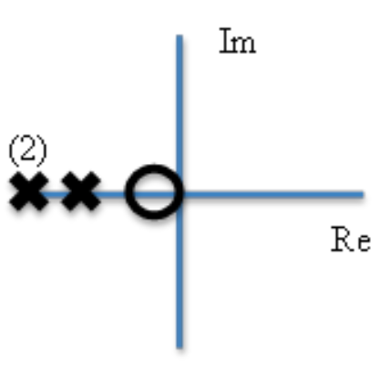
We solve for the s values. For the numerator, s = -0.5, which corresponds to a zero. For the denominator, s = -3 (double), -2, which corresponds to poles. The plot below shows how we should plot this.

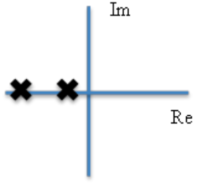
a graph with real x-axis and imaginary y-axis. There are two xes along the x-axis at (-3,0) and (-2,0). There is a number two above the x at (-3,0), indicating a double pole. There is a circle at (-0.5,0), indicating a zero.

If all of the poles are in the left-hand plane, the system is stable. This means that it has negative real numbers and may or may not have an imaginary value as shown in the graph below. If the pole is all real numbers, the system will be a decaying exponential. If the pole is a complex number, the system will be an oscillating decay. Both are stable.

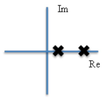
a graph with real x-axis and imaginary y-axis. There are two xes along the negative x-axis, indicating two poles in the left-hand plane.

If any of the poles are in the right-hand plane, the system is unstable. This means that at least one pole has a positive real number and may or may not have an imaginary value as shown in the graph below:

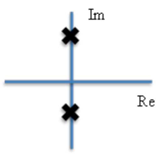
a graph with real x-axis and imaginary y-axis. There are two xes along the positive x-axis, indicating two poles in the right-hand plane.

If any of the poles are on the imaginary y-axis, the system is marginally stable. This means that at least one pole has a real value of 0 and may or may not have an imaginary value as shown in the graph below:

a graph with real x-axis and imaginary y-axis. There are two Xes along the imaginary y-axis, indicating two poles along the y-axis.