Current page:

Fourier Transform and Frequency Domain

Introduction

Though the time domain is an intuitive and useful way to study signals, it can be difficult to discern all characteristics of complicated signals this way. When signals increase in complexity and contain sine waves of multiple frequencies, amplitudes, and offsets, don’t seem to repeat regularly, and last for a long time, traditional time domain methods to analyse signals fail to fully describe the signal.

This is when performing a fourier transform becomes very valuable. It allows us to break down complicated signals into its component sine waves with defined amplitudes and frequencies. This page will discuss the mathematics behind performing a fourier transform manually, and the information that we can get out of it.

Fourier Transform

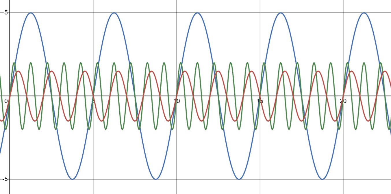
Recall that we can approximate any signal as a combination sum of an infinite number of sinusoids. Using this as a basis, we can represent our signals as a series of sinusoids with various frequencies, amplitudes, and phase delays that constructively or destructively interfere to produce patterns that exist in the time domain signal. These are important, as they represent the characteristics of the initial signal, and will help us later in figuring out the output.

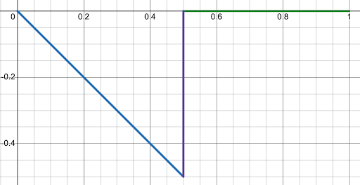
We do so through the following equation:

Fourier Transform Equation

$$ H(\omega) = \int_{-\infty}^\infty f(t)e^{-j2\pi\omega t} dt $$

Example Problem: Solving for Fourier Series Coefficients #undefined

Find the magnitude and frequency plot, the first four Coefficients, and $ C_0 $, $ C_m $, and $ 0_m $ for these coefficients.

$ x(t)= \begin{cases} &-t,\ t<0.5\\ &0,\ 0.5\leq t<1\\ \end{cases} $

Begin with the equation for $ b_m $:

$ b_m = \frac{2}{T}\int_0^Tx(t)sin(2mf_1t\pi)dt $

Frequency Domain

Fourier transforms allow us to plot signals in the frequency domain. Frequency domain or Fourier plots show us the amplitude of every frequency of sinusoid that makes up a signal.

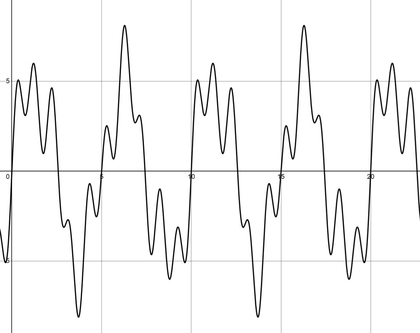
Figure 1. A time domain plot. The blue signal has a frequency of 0.2Hz and an amplitude of 5V. The red signal has a frequency of 0.5Hz and an amplitude of 1.5V. The green signal has a frequency of 1Hz and an aplitude of 2V.

Figure 2. The linear combination of the three signals above. Many biological signals overlap like this.

As multiple frequencies overlap within one signal, it becomes more and more difficult to discern the individual characteristics of each frequency. The signal looks messy now and its attributes cannot be easily determined by eye.

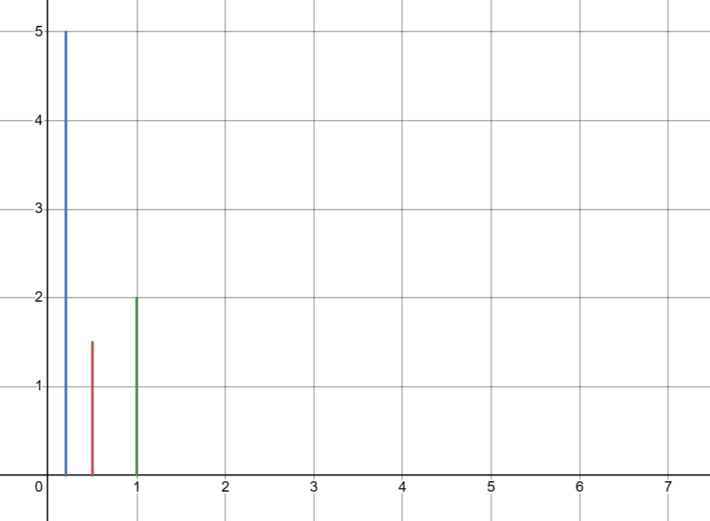
Figure 3. A frequency domain plot of the time domain signal above, the x-axis now represents frequency in Hz.

Notice that the three peaks still describe the amplitude and frequency of the signals in Figure 1. There are only three straight lines because no noise and no other frequencies are present. No matter how messy a signal looks in the time domain, the frequency domain plot easily decomposes the signal into its component parts. When noise and non-discrete frequencies are added, frequency domain plots can look messy too, but more tools exist to interpret frequency plots such as power spectrum, bode plots, and filters.

By breaking down a signal this way, we are able to identify frequencies with large amplitudes that influence the signal a lot, or components of noise that might be filtered out. This domain is the most useful for assessing what the impact of transformations from systems may have, and allow us to simplify math when we do convolutions.