Laplace Transform
What Are Laplace Transformations?
This is another frequency mapping technique that can be easier to use than the Fourier Transforms as these use a table and map certain identities to known transforms. Laplace transforms are used to describe transfer functions since laplace domain makes transfer function maths a lot easier. When a signal is affected by a transfer function, the input is simply multiplied by the transfer function to produce the output which is a much simpler operation to complete than convolution in the time domain.
Quick Facts About Laplace Transforms
Laplace Transforms:
- Are linear.
- Uses "s" as its variable, a complex numnber.
- Require initial conditions.
- Can be done forwards and backwards (or in inverse) without losing information
| Time Domain: f(t) | Laplace Domain: F(s) |
|---|---|
| Impulse \( \delta(t) \) | \( 1 \) |
| Step \( 1(t) \) | \( \frac{1}{s} \) |
| Ramp \( t \) | \( \frac{1}{s^{2}} \) |
| \( t^{n} \) | \( \frac{n!}{s^{n+1}} \) |
| \( e^{-at} \) | \( \frac{1}{s+a} \) |
| \( te^{-at} \) | \( \frac{1}{(s+a)^2} \) |
| \( \sin(\omega t) \) | \( \frac{\omega}{s^2+\omega^2} \) |
| \( \cos(\omega t) \) | \( \frac{s}{s^2+\omega^2} \) |
| \( e^{-at}\sin(\omega t) \) | \( \frac{\omega}{(s+a)^2+\omega^2} \) |
| \( e^{-at}\cos(\omega t) \) | \( \frac{s+a}{(s+a)^2+\omega^2} \) |
Where \( t \geq 0 \) for all time domain functions.
Common Signals In Laplace Domain
| Function | Plot | Time Domain: f(t) | Laplace Domain: F(s) |
|---|---|---|---|
| Step | 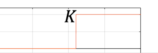 | \( x(t) \begin{cases} &0\ \ \ \ t\leq 0\\ &K\ \ \ t>0\\ \end{cases} \) | \( \frac{K}{s} \) |
| Ramp | 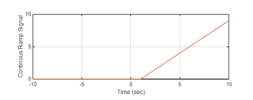 | \( r(t) \begin{cases} &0\ \ \ \ \ \ t\leq 0\\ &Kt\ \ \ t>0\\ \end{cases} \) | \( \frac{K}{s^2} \) |
| Impulse | 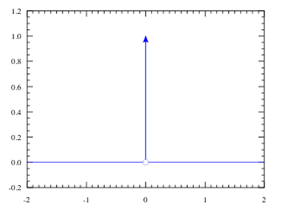 | \( \delta(t) \) | \( 1 \) |
| Pulse/Rectangle | 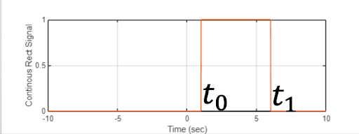 | \( rect(t) = \begin{cases} &1\ \ \ t_0<t<t_1\\ &0\ \ \ else\\ \end{cases} \) | \( \frac{1}{s}-\frac{e^{-t_{1}s}}{s} \) |
Laplace Transform With Other Domains
| Time ==> Laplace | Laplace Transform |
| Laplace ==> Time | Inverse Laplace Transform |
| Laplace ==> Frequency | Steady State \( s = j\omega \) |
| Frequency ==> Laplace | No Initial Conditions \( j\omega = s \) |