Stability

What Is Stability?

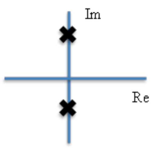
When we have a system, there are three outcomes: stable, unstable, and marginally stable. Stable means that the system reaches a steady state, whereas unstable describes a system that explodes to infinity. Marginally stable is a distinct case where the system does not reach a steady state but remains bounded, such as a sinusoid.

Determining System Stability From Graphs

Using the Laplace transfer function, we can plot the poles and zeros on the complex s-plane, where the x-axis represents the real values and the y-axis represents imaginary values. For example, consider the equation:

$$ G(s) = \frac{s+0.5}{(s+3)^{2}(s+2)} $$

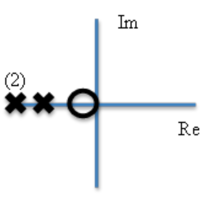
We solve for the s values. For the numerator, s = -0.5, which corresponds to a zero. For the denominator, s = -3 (double), -2, which correspond to poles. The plot below shows how we should plot this.

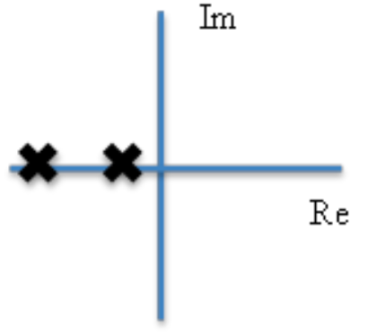
a graph with real x-axis and imaginary y-axis. There are two xes along the x-axis at (-3,0) and (-2,0). There is a number two above the x at (-3,0), indicating a double pole. There is a circle at (-0.5,0), indicating a zero.

If all of the poles are in the left half-plane (LHP), the system is stable. This means that each pole has a negative real part and may or may not have an imaginary component as shown in the graph below. If a pole is purely real, the system response is a decaying exponential. If a pole is a complex number with a negative real part, the system exhibits oscillatory decay. Both are stable.

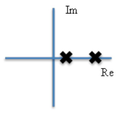
a graph with real x-axis and imaginary y-axis. There are two xes along the negative x-axis, indicating two poles in the left-hand plane.

If any of the poles are in the right half-plane (RHP), the system is unstable. This means that at least one pole has a positive real part and may or may not have an imaginary component as shown in the graph below:

a graph with real x-axis and imaginary y-axis. There are two xes along the positive x-axis, indicating two poles in the right-hand plane.

If any of the poles lie on the imaginary axis (with a real value of 0) and are not repeated, the system is marginally stable, as shown in the graph below:

a graph with real x-axis and imaginary y-axis. There are two Xes along the imaginary y-axis, indicating two poles along the y-axis.